How to nail uncertainty calculations in IB Physics

State results as value ± uncertainty. Add absolute uncertainties for sums and differences, add percentage uncertainties for products and divisions, and multiply percentage uncertainty by the power when raising a quantity to n. That single rule set covers most of what IB Physics asks of you, both in the lab and in Paper 1 and Paper 2 questions.

Before you go further, here’s the working checklist:

• For repeated readings, use half the range (max minus min, divided by two) as your absolute uncertainty for small data sets, or the standard error (standard deviation ÷ √n) once you have enough repeats to justify it.
• For a single reading, use ±half the smallest division on an analogue instrument, or the manufacturer’s stated resolution for a digital one.
• Addition or subtraction of measured quantities: add the absolute uncertainties.
• Multiplication or division: add the percentage uncertainties.
• A quantity raised to a power n: multiply its percentage uncertainty by n.

Key Takeaways

Uncertainty calculations in IB Physics rest on three propagation rules: add absolute uncertainties for sums, add percentage uncertainties for products or divisions, and multiply percentage uncertainty by the power for exponents.

Point	Details
Estimating uncertainty	Use half-range for a few repeats, standard error for many, and half the smallest division for a single reading.
Propagation rules	Add absolute for +/−, add percentage for ×/÷, and multiply percentage by the power for exponents.
Rounding convention	Round the uncertainty to one significant figure, then match your value’s precision to it.
Gradient uncertainty	Use Δgradient = (steepest line minus shallowest line) ÷ 2 from a max/min best-fit approach.
Practise with Tiber Tutor	Examiner-authored topic tests and mock exams on Tiber Tutor track exactly where you lose marks on propagation steps.

Table of Contents

• Understanding uncertainty calculations in IB Physics: the core types
• Converting between absolute, fractional and percentage uncertainty
• Propagating uncertainty through a calculation
• Getting uncertainty right on graphs: gradients and intercepts
• Worked examples: three calculations you’ll actually meet
• What examiners actually reward, and where students lose marks
• How Tiber Tutor helps you practise uncertainty calculations
• Where uncertainty calculations stop being reliable
• Where uncertainty actually creeps into your IB Physics practicals
• Uncertainty and error are not the same thing
• Reporting uncertainties well in your lab report
• An exam-time checklist worth memorising
• Practise uncertainty questions with examiner-built topic tests
• Sources
• FAQ

Understanding uncertainty calculations in IB Physics: the core types

Every measurement carries some doubt, and IB Physics wants you to quantify it in three specific forms. Absolute uncertainty (Δx) has the same units as the measurement itself, e.g. 25.0 ± 0.5 cm. Fractional uncertainty is Δx/x, a plain number with no units. Percentage uncertainty is (Δx/x) × 100%, the form examiners usually want in your final answer.

Uncertainty also splits by cause. Random uncertainty scatters your readings above and below the true value, usually from reaction time, parallax, or fluctuating conditions, and repeating the measurement reduces its effect. Systematic uncertainty shifts every reading the same way, such as a zero error on a newton meter, and no amount of repetition fixes it. Metrologists label these more formally as Type A (evaluated statistically from repeated readings) and Type B (evaluated from instrument specifications or prior knowledge), a distinction the NIST guide on measurement uncertainty sets out clearly.

For estimating uncertainty on real apparatus:

• Analogue scale, single reading: ±half the smallest division.
• Digital display: ±1 in the last displayed digit, unless the manual states otherwise.
• Repeated trials (3 to 5): half-range is the pragmatic choice.
• Repeated trials (6 or more): standard error becomes statistically meaningful.

Pro Tip: Don’t default to standard error just because it looks more rigorous. With only three or four repeats, half-range is the honest choice, and examiners know it.

Converting between absolute, fractional and percentage uncertainty

You’ll move between these three forms constantly, so the conversions need to be automatic rather than something you derive under exam pressure.

1. Absolute uncertainty (Δx): stated directly from your measurement, e.g. length = 12.4 ± 0.1 cm.
2. Fractional uncertainty: Δx ÷ x. For the example above, that’s 0.1 ÷ 12.4 = 0.0081.
3. Percentage uncertainty: fractional uncertainty × 100. Here, 0.0081 × 100 = 0.81%.
4. Reverse conversion: if you’re given a percentage uncertainty, multiply it by the measured value and divide by 100 to recover the absolute uncertainty.

Rounding matters more than most students think. The convention is to round the uncertainty itself to one significant figure (two only if the leading digit is 1), then match your measured value’s decimal places to that uncertainty, a practice detailed in IB revision guidance on measurement and uncertainties. So 12.437 ± 0.0623 becomes 12.44 ± 0.06, not 12.437 ± 0.0623.

Before you finalise any answer, run this checklist:

1. Have I quoted the uncertainty to one significant figure?
2. Does my measured value’s precision match that uncertainty’s decimal place?
3. Have I included units on the absolute uncertainty, and no units on the percentage form?
4. Have I checked whether the question wants absolute, fractional, or percentage uncertainty specifically?

Propagating uncertainty through a calculation

Once you have uncertainties on your raw measurements, you need rules for combining them when those measurements feed into a formula. IB Physics tests four scenarios repeatedly, and each has its own shortcut.

• Addition or subtraction (y = a + b or y = a − b): add the absolute uncertainties, Δy = Δa + Δb, regardless of whether the operation is a plus or a minus.
• Multiplication or division (y = a × b or y = a ÷ b): add the percentage uncertainties, Δy% = Δa% + Δb%.
• Powers (y = xⁿ): multiply the percentage uncertainty by the power, Δy% = n × Δx%. A radius squared in an area formula doubles its percentage uncertainty; a radius cubed in a volume formula triples it.
• Independent random uncertainties, more rigorous treatment: combine in quadrature, √((Δa)² + (Δb)²), which gives a statistically valid result rather than the pessimistic worst-case figure simple addition produces.

A practical shortcut worth knowing: when one uncertainty contributes more than three times the next largest, the University of North Carolina’s uncertainty guide notes you can often treat that dominant term as the combined uncertainty without materially changing your answer. This saves real time in a 90-minute Paper 3 session, provided you state the assumption in your working.

For non-linear functions like sine, cosine, or logarithms, none of these simple rules apply cleanly. That’s where the maximum-minimum method, or full Monte Carlo propagation for advanced work, becomes the safer route rather than an approximation that quietly misleads you.

Getting uncertainty right on graphs: gradients and intercepts

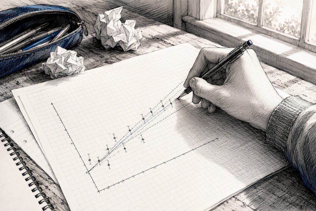
Error bars turn a scatter of points into something you can actually interrogate. You rarely need to plot one on every single point either; IB examiners generally accept error bars on the first and last points, or on whichever point looks the most anomalous, provided your reasoning is visible.

1. Plot your data points with vertical error bars sized to the uncertainty on the dependent variable (and horizontal bars if the independent variable’s uncertainty is significant).
2. Draw your best-fit line through the points as normal.
3. Draw the steepest acceptable line that still passes through every error bar, then the shallowest acceptable line that does the same.
4. Calculate the gradient of each: Δgradient = (gradient max − gradient min) ÷ 2.
5. Read the intercepts of the max and min lines off the y-axis, then apply the same halving formula to get the intercept’s uncertainty.

Report your final gradient as gradient ± Δgradient, and your intercept the same way, both rounded consistently with the significant-figure rule from earlier.

Pro Tip: If your steepest and shallowest lines both pass through every error bar comfortably, your error bars are probably too generous. A well-calibrated uncertainty should make the max/min lines feel like they’re only just managing to fit.

Worked examples: three calculations you’ll actually meet

These three scenarios cover most of what appears across IB Physics practicals and Paper 3 data-analysis questions.

Example 1: single instrument reading. A ruler with 1 mm divisions gives a length of 15.6 cm. Absolute uncertainty = ±half the smallest division = ±0.05 cm. Report as 15.60 ± 0.05 cm.

Example 2: repeated measurements. Five timings of a pendulum swing give 2.01, 2.05, 1.98, 2.03, 2.00 s. Mean = 2.014 s. Range = 2.05 − 1.98 = 0.07 s, so half-range = 0.035 s, rounded to one significant figure gives 2.01 ± 0.04 s.

Example 3: a derived quantity. You calculate momentum p = mv, with mass 0.500 ± 0.002 kg and velocity 3.20 ± 0.10 m/s.

What examiners actually reward, and where students lose marks

Examiners award method marks for showing your propagation steps clearly, even when your final rounding isn’t perfect. A visible line of working, “percentage uncertainty in v = (0.10/3.20) × 100 = 3.1%”, earns credit that a bare final answer never will.

The recurring mistakes are predictable:

• Mixing significant figures between the value and its uncertainty, e.g. quoting 15.637 ± 0.05 rather than 15.64 ± 0.05.
• Skipping the propagation step entirely and guessing a final uncertainty.
• Treating a systematic error, like a zero offset, as though repeating the measurement would reduce it.
• Forgetting units on absolute uncertainty while quoting them on a percentage figure.

Present your final result on one clear line, value ± uncertainty with correct units, and where the question asks for it, a brief comment on whether your result agrees with theory within the stated uncertainty range.

How Tiber Tutor helps you practise uncertainty calculations

Reading the rules is one thing; applying them under time pressure on unfamiliar data is another. Tiber Tutor’s IB Physics topic tests include uncertainty and propagation questions built with examiner-style mark schemes, so you see exactly where marks are awarded for showing method.

• Personalised analytics flag whether you’re consistently losing marks on the propagation step rather than the final arithmetic.
• Cram sheets, animated videos, and worked exemplars interlink directly with each topic test, so a shaky gradient-uncertainty question links straight back to the relevant notes.
• Mock exams let you rehearse full data-analysis questions at Paper 3 pace, not just isolated formulae.

Where uncertainty calculations stop being reliable

The rules covered so far work well for linear combinations of independent, well-behaved measurements, but they quietly break down in a few situations worth knowing about before you lean on them in an IA.

Simple percentage addition assumes each source of uncertainty is independent and roughly comparable in size. When one term dominates heavily, the addition rule can overstate the combined uncertainty, which is why the largest-term shortcut exists. Quadrature (root sum of squares) gives a more statistically defensible answer for genuinely independent random uncertainties, corresponding to roughly a 68% confidence interval, as NIST’s guidance on propagating measurement uncertainty explains. Simple addition, by contrast, gives a worst-case bound that’s usually wider than necessary.

Non-linear functions cause the bigger problem. Trigonometric relationships, logarithms, and anything where the output is highly sensitive to small input changes near a turning point can make the standard percentage rules mislead you, particularly for angles near 0° or 90° where sine or cosine curves flatten out. In these cases, the maximum-minimum method, calculating the result at the extreme values of each input, gives a safer bound than blindly applying percentage propagation.

There’s also a ceiling on how much precision uncertainty calculations can actually deliver. If your systematic uncertainty hasn’t been identified at all, no amount of careful propagation on the random component will produce an accurate final figure. Propagation only ever accounts for the uncertainties you’ve actually included in your budget. For most IB assessments, the classroom rules are entirely sufficient. For an IA chasing a higher level of rigour, presenting an uncertainty budget table listing each Type A and Type B contribution separately demonstrates the kind of understanding that stands out, and tools like the NIST Uncertainty Machine exist for exploring this further if you’re curious.

Where uncertainty actually creeps into your IB Physics practicals

Every practical has its own fingerprint of uncertainty sources, and recognising them quickly is half the battle in a written evaluation section.

Timing experiments (pendulums, terminal velocity, decay simulations) suffer mostly from human reaction time, typically around 0.2 seconds for a stopwatch start and stop. This is why timing multiple oscillations and dividing, rather than timing one, is standard IB practice.

Length and distance measurements run into parallax error when you read a scale from an angle, plus the resolution limit of the ruler or vernier calliper itself. A metre rule with obscured end markings adds a systematic uncertainty you won’t spot unless you check the zero point.

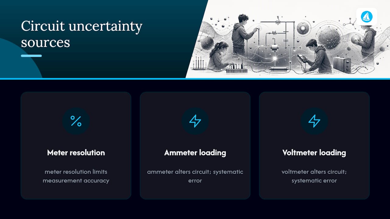
Electrical circuits carry uncertainty from meter resolution, but also from ammeter and voltmeter loading effects, where the meter itself slightly alters the circuit it’s measuring, a systematic effect students frequently mislabel as random noise.

Temperature measurements are vulnerable to thermal lag, the delay between the true temperature change and the thermometer catching up, plus heat loss to the surroundings during a heating experiment. Both are systematic and won’t average out no matter how many repeats you take.

Optical experiments (refraction, diffraction, lens focal length) are dominated by the difficulty of judging exactly where a faint or spread-out image forms, which inflates the effective resolution uncertainty well beyond the ruler’s smallest division.

Spotting which category your practical falls into, and naming the specific mechanism rather than writing “human error”, is what separates a strong evaluation section from a generic one.

Uncertainty and error are not the same thing

Students conflate these terms constantly, and it costs marks in evaluation sections. Error is the difference between a measured value and the true (or accepted) value. It’s a single number you can sometimes calculate retrospectively, once you know or can look up the accepted value, but you can never know it with certainty for a genuinely unknown quantity.

Uncertainty is your estimate of the range within which the true value probably lies, calculated before you know whether your result is even close to correct. It reflects the limitations of your method and equipment, not a comparison against a known answer.

Here’s where it gets practical: you can have a large uncertainty and a small error, if you got lucky. You can equally have a tiny uncertainty and a huge error, if a systematic problem, like a miscalibrated instrument, shifted every reading the same way. A percentage difference calculation, comparing your result to a textbook value, tells you about error. A propagation calculation, following the rules covered earlier in this guide, tells you about uncertainty. Mixing the two up in your evaluation, claiming your uncertainty “proves” your result is accurate, is one of the more common conceptual mistakes examiners flag.

Reporting uncertainties well in your lab report

A results section that handles uncertainty properly reads differently from one that bolts it on as an afterthought, and examiners notice the difference immediately.

State every measured value as value ± absolute uncertainty, with consistent units and matching decimal places, right from your raw data table onward, not just in your final answer. Round the uncertainty to one significant figure before you round the value to match. Include a column in your data table for uncertainty rather than mentioning it once in a footnote.

When you calculate a derived quantity, show the propagation step explicitly. Write out “percentage uncertainty in v = …” rather than jumping straight to a final ± figure with no visible working. This single habit accounts for a disproportionate share of lost method marks.

Distinguish random from systematic sources in your evaluation, and suggest specific, mechanism-based improvements rather than vague ones. “Use a light gate instead of manual timing to remove reaction-time uncertainty” earns more credit than “be more careful”. For an IA aiming at the top mark bands, an uncertainty budget table separating Type A and Type B contributions signals a level of rigour examiners are specifically looking for.

Finally, comment on whether your final result agrees with any accepted or theoretical value within your stated uncertainty range, phrased as a genuine comparison rather than a throwaway line. That comparison is often the single sentence that separates a mediocre conclusion from a strong one.

An exam-time checklist worth memorising

Under time pressure, five checks cover most of what goes wrong. State every result as value ± uncertainty, with units on the absolute form only. Choose the correct propagation rule (add absolute for sums, add percentage for products, multiply percentage by the power) before you touch a calculator. Round your uncertainty to one significant figure first, then match your value to it.

For an IA, keep your full working visible, including intermediate percentage uncertainties. In an exam, present the same logic more concisely, but never skip the step entirely. If you only remember one thing, remember that the propagation rule you choose depends on the operation, not on which numbers look messier.

Rehearsing this under timed conditions matters more than reading it once. Practising with realistic data sets on IB Physics mock exams is the difference between knowing the rules and applying them fluently when the clock is running.

— Oliver

Practise uncertainty questions with examiner-built topic tests

Tiber Tutor is is built specifically around what IB examiners reward, because actual IB examiners write the content. That matters most on a topic like uncertainty, where the difference between a 6 and a 7 often comes down to whether your propagation working is visible and correctly structured, not whether your final number is exact.

The platform’s IB Physics topic tests target uncertainty and propagation questions directly, each mapped to an examiner-style mark scheme so you see precisely where marks are gained or lost. Every test links to cram sheets and worked video exemplars covering the same syllabus point, so a weak answer on gradient uncertainty leads you straight back to the explanation rather than leaving you guessing. Personalised analytics then track whether your errors cluster around propagation steps, rounding, or presentation, something a static worksheet or PDF simply cannot show you. Start with a topic test on measurement and uncertainty, check your analytics, then move on to a full mock exam once you’re consistently showing clean working.

Sources

For deeper technical grounding beyond IB scope, the NIST Simple Guide to measurement uncertainty and the NIST Uncertainty Machine cover full metrology procedures, including Monte Carlo propagation.

• Simple Guide for Evaluating and Expressing the Uncertainty of NIST Measurement Results
• Uncertainty guide — UNC

FAQ

How do you calculate uncertainty in IB Physics?

State your measurement as value ± absolute uncertainty, using half the range for repeats or half the smallest division for a single reading, then apply the addition, percentage, or power rule depending on the calculation.

When should you use range/2 instead of standard error?

Use half-range for small data sets of three to five repeats; switch to standard error (standard deviation ÷ √n) once you have six or more readings for a statistically meaningful result.

How many significant figures should an uncertainty have?

Round the uncertainty to one significant figure, or two if the leading digit is 1, and match your measured value’s decimal places to that uncertainty.

How do you find the uncertainty in a gradient?

Draw the steepest and shallowest acceptable lines through your error bars, then calculate Δgradient = (steepest gradient minus shallowest gradient) ÷ 2.

What is the difference between uncertainty and error?

Error is the gap between your measured value and the true value; uncertainty is your estimated range for where the true value probably lies, calculated independently of whether your result is actually accurate.

Where can I practise uncertainty questions with mark schemes?

Tiber Tutor’s IB Physics topic tests include uncertainty and propagation questions built with examiner-style mark schemes, plus personalised analytics showing where marks are typically lost.

Recommended

• IB Physics Tests » Tiber Tutor
• IB Physics Exam Format Explained: 2026 Guide For Students » Tiber Tutor
• IB Physics Custom Test » Tiber Tutor